Back in July I wrote a post about thinking beyond localized activations, and in August I showed the gain that comes from sharing one learnable activation globally: a single nonlinearity, shared by every layer and learned alongside the weights, outperforms a fixed GELU at ImageNet-1K scale. This post picks up from there. Because the shared function is one object rather than a scatter of per-layer curves, it can be frozen after training and installed in a different network.
Some of the evidence below is also available as an interactive page — hover a cell for its numbers, isolate a curve, switch datasets. Links sit in the sections they belong to; the first is the hyperparameter search landscape under “You just got lucky with the learning rate”. There is also a figure explorer for the whole paper — every figure and table as a live chart, with sliders on the five coefficients, an epoch scrubber, per-seed toggles and zoom.
A network’s activation function is normally a fixed design choice — you pick GELU, bolt it after every layer, and gradient descent takes care of the rest. Instead, give the entire network one activation function, described by five numbers, and learn those five numbers along with the weights. On ImageNet-1K this is worth about two points of top-1 over GELU. Then freeze the five numbers, drop them into a completely different, much smaller network, and they keep working — beating ten conventional activation functions on four datasets.
We call it FAct, for Fourier Activation.
The assumption worth poking
There is no activation function that is consistently the best one. ReLU, LeakyReLU, ELU, SELU, Softplus, tanh, GELU, SiLU, Mish, HardSwish — the field has produced a long list, some designed by hand and some found by search, and which of them wins depends on the model and the task.
The obvious response is to make the activation learnable, and plenty of people have: PReLU learns the negative slope, and richer parameterizations (APL, ACON, rational/Padé units, kernel activations) let more of the curve move. But look at where those parameters live. They are attached to individual neurons, to channels, or at best to a layer. A trained network ends up holding many curves, and no single one of them is “the network’s nonlinearity.”
That closes off a possibility that seems worth having open: learning one nonlinearity for a whole network, and then reusing it in a different network. If the learned function is a per-layer artifact, there is nothing to lift out. If it is a network-level component, there is.
FAct: one parameter set, every hidden layer
Let $z_l$ be the pre-activation at hidden layer $l$, and $\phi(z;\theta)$ the activation parameterized by $\theta$. FAct uses a single $\theta$ everywhere:
\[h_l \;=\; \phi(z_l;\theta), \qquad l = 1,\ldots,L .\]That one line is the entire architectural change. Its consequence is in the backward pass: because the same parameters are used at every hidden layer, their gradients aggregate over the whole network.
\[\frac{\partial \mathcal{L}}{\partial \theta} \;=\; \sum_{l=1}^{L} \frac{\partial \mathcal{L}}{\partial \phi(z_l;\theta)}\, \frac{\partial \phi(z_l;\theta)}{\partial \theta} .\]The curve is not shaped by what one layer wants. It is shaped by what every block wants, summed. And after training, there is exactly one function to point at — so it can be frozen and installed elsewhere.
Two names for the two settings, used throughout: Learnable FAct is the function being optimized jointly with the source network, Frozen FAct is that same function afterwards, held fixed inside a different network.
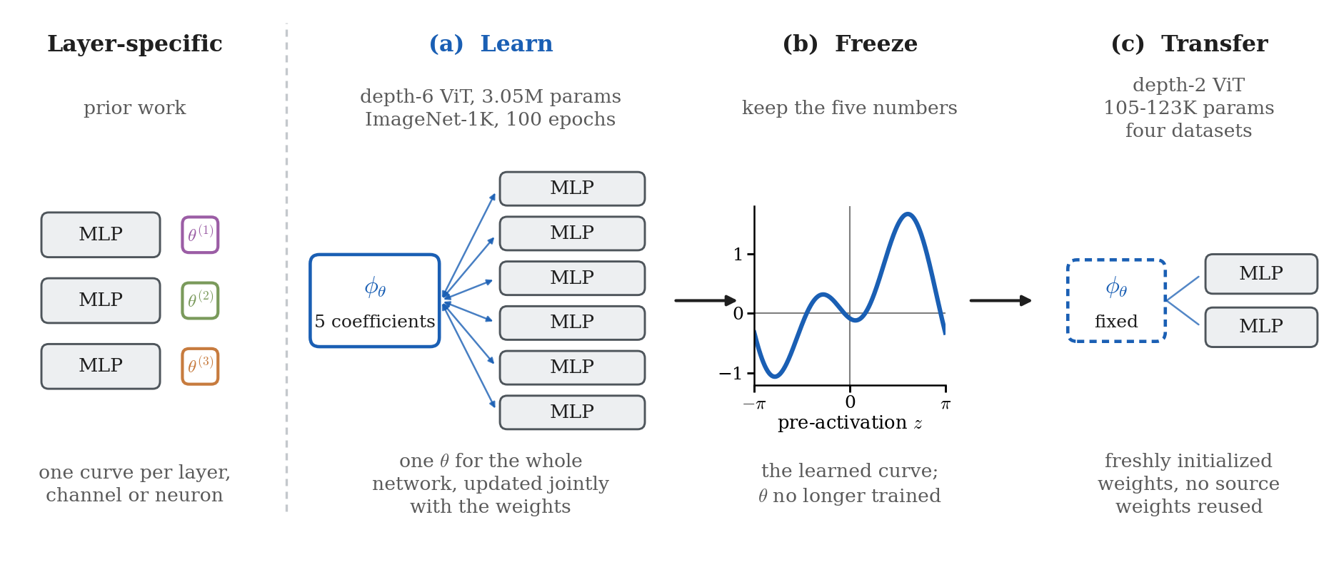
Left, for contrast: conventional learnable activations attach parameters to layers, channels or neurons. (a) FAct instantiates one parameter set, five coefficients total, and every feed-forward block of the source network applies the same function; the coefficients receive gradients from every block. (b) After source training the five coefficients are frozen. (c) The frozen function is installed as an ordinary fixed activation in a smaller, independently initialized target network, which receives no weights from the source model.
Why a Fourier basis
If one function has to serve every hidden layer, the parameterization had better be able to express a lot. Conventional activations span monotonic, non-monotonic, bounded, unbounded and oscillatory families; a restricted parameterization quietly decides in advance which of those the shared function is allowed to be.
There is also a hint in the literature that nobody chased. In the activation search that produced Swish, Ramachandran et al. report that the search kept turning up functions built from $\sin$ and $\cos$ — candidates like $\cos(z) - z$ and $\min(z, \sin z)$ — and note that periodic activations had been “only briefly explored,” calling it a fruitful route for further research. Nobody took it very far.
So we use a truncated Fourier series:
\[\phi(z;\theta) \;=\; a_0 + \sum_{k=1}^{K}\big[\, a_k\cos(k\omega z) + b_k\sin(k\omega z) \,\big], \qquad \theta = \{a_0\} \cup \{a_k, b_k\}_{k=1}^{K} .\]with $\omega = 1$ fixed in every experiment, so the period is $2\pi$ and $\theta$ is just the $2K{+}1$ coefficients. $\omega$ is a constant of the parameterization, not something we learn.
Two properties matter here, and the second one is easy to miss:
It can change shape, not just a region. Unlike parameterizations that adjust one branch of a predefined activation, combining harmonics lets the overall shape of the curve move during optimization.
It is bounded by the sum of the magnitudes of its coefficients. This is exactly the property you want under global sharing. Different layers occupy different pre-activation ranges, and a shared function must not blow up at a value that only some of them reach. The function we end up transferring is bounded by 2.185 on the whole real line — so a target network that produces pre-activations the source model never saw still cannot drive the activation to a large output. A rational parameterization has no such guarantee; the Swish search itself reported that candidates using division tend to do badly because the output explodes when the denominator approaches zero.
We use $K = 2$ in the main experiments. Five scalars define the nonlinearity of every hidden unit of every block — five for the whole network, not five per unit.
Starting from GELU and walking away from it
FAct is initialized at the Fourier coefficients of GELU on one period. Writing $\sigma$ for the reference activation,
\[a_0=\frac{1}{2\pi}\!\int_{-\pi}^{\pi}\!\sigma(z)\,dz,\quad a_k=\frac{1}{\pi}\!\int_{-\pi}^{\pi}\!\sigma(z)\cos(k\omega z)\,dz,\quad b_k=\frac{1}{\pi}\!\int_{-\pi}^{\pi}\!\sigma(z)\sin(k\omega z)\,dz ,\]which for GELU at $K = 2$ and $\omega = 1$ gives
\[a_0 = 0.7061,\quad a_1 = -0.7049,\quad a_2 = 0.0261,\quad b_1 = 1.0000,\quad b_2 = -0.5000 .\]This is a truncated representation of GELU, not GELU itself — the familiar starting point, with nothing holding it there.
By the end of 100 epochs on ImageNet-1K the five numbers are
\[a_0 = 0.2182,\quad a_1 = 0.1193,\quad a_2 = -0.4237,\quad b_1 = 0.8315,\quad b_2 = -0.5918 .\]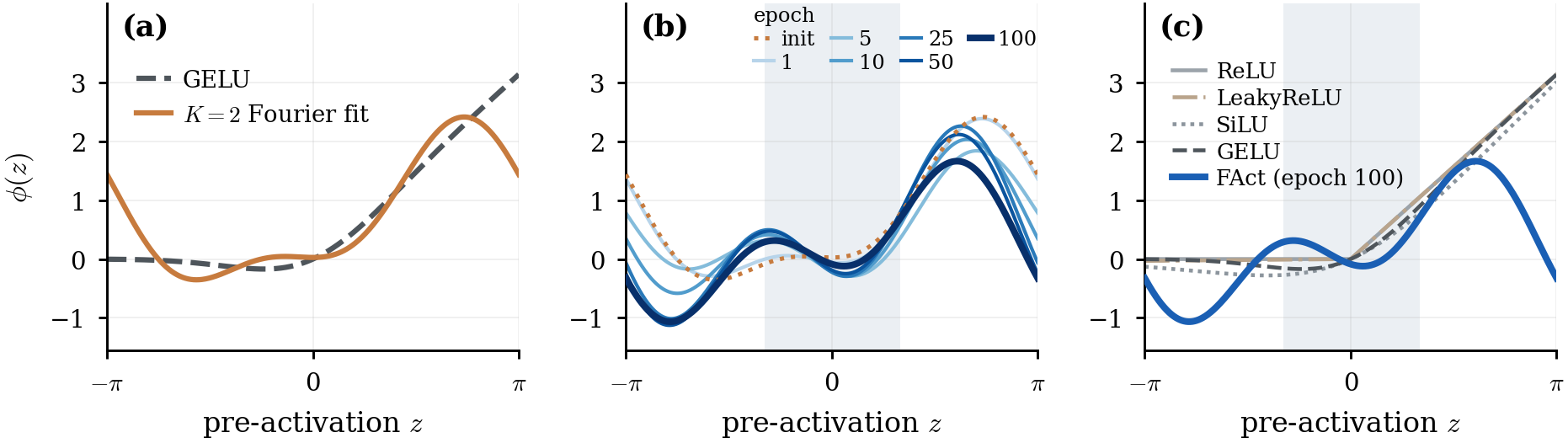
(a) GELU against the $K{=}2$ Fourier series used to initialize FAct. (b) The shared curve at epochs 1, 5, 10, 25, 50 and 100, initialization dotted; the shaded band is the central 98% of the source model’s pooled pre-activations, $[-1.03, 1.05]$, measured at every activation site over 512 held-out images. (c) The epoch-100 curve — the one that gets frozen — against four fixed activations.
Three things about that curve are worth stating plainly:
- It is not a familiar function. It has four critical points in the period, at $z = -2.46,\ -0.87,\ 0.19$ and $1.91$, and two of them fall inside the band that holds the central 98% of the source model’s pre-activations. It is non-monotonic, and it turns downward before the end of the period. None of the fixed activations do that. Whatever optimization is doing here, it is not rediscovering GELU.
- Most of the motion is early. The bulk of the change happens in the first ten epochs and the curve is close to settled by epoch 50.
- It is not a fluke of one run. Over the three seeds for which coefficient trajectories were recorded, the largest disagreement in any of the five coefficients at the end of training is 0.017. Different seeds walk to the same place.
Does it help? ImageNet-1K
The source model is ViT-d6 — a depth-6, 3.05M-parameter Vision Transformer at 224×224, patch 16 — trained for 100 epochs on ImageNet-1K. Five seeds each for FAct and GELU.
| Activation | Learnable | Seeds | Test top-1 (%) | Validation AUC (%) |
|---|---|---|---|---|
| Learnable FAct | yes | 5 | 64.38 ± 0.44 | 55.92 ± 0.41 |
| GELU | no | 5 | 62.45 ± 0.13 | 53.84 ± 0.11 |
| ReLU | no | 1 | 60.92† | 52.37† |
| LeakyReLU | no | 1 | 60.91† | 52.24† |
| SiLU | no | 1 | 60.72† | 51.59† |
| Mish | no | 1 | 60.36† | 51.88† |
† single-seed arm. Validation AUC is the epoch-weighted mean validation top-1 over the run — a summary of the whole trajectory rather than its endpoint.
Seed-matched, the gain over GELU is +1.93 ± 0.43 pp ($t = 10.02$, $p = 5.6\times10^{-4}$, five seeds).
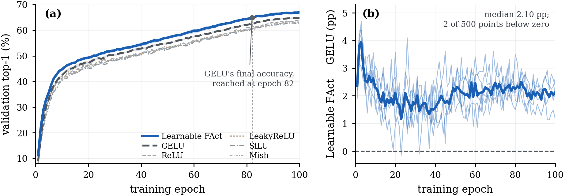
(a) Validation top-1 against epoch. FAct and GELU are 5-seed means with a ±1 s.d. band; the other four are single runs, drawn thin. (b) The seed-matched difference FAct − GELU at every epoch: five thin lines, one per seed, and their mean in bold.
It is not an endpoint effect. The mean FAct curve is above GELU’s at every one of the 100 epochs, only 2 of the 500 seed–epoch points fall below zero, and FAct reaches GELU’s end-of-training validation accuracy at epoch 82 — an 18% saving in epochs. The AUC gap (55.92 vs 53.84) says the same thing: the advantage is spread across training, not concentrated at the end.
Freeze it, and put it in a different network
This is the part the whole design was for. Take the five numbers from the ImageNet run, freeze them, and install them as an ordinary fixed activation in ViT-d2 — a depth-2 Vision Transformer with embedding dimension 64 and 105–123K parameters, 25 to 29× smaller than the source depending on the dataset, freshly initialized. No weights are transferred. The activation parameters are not updated during target training. Different depth, different width, different datasets, different task.
Mean test accuracy over six seeds, common training configuration:
| Activation | Fashion-MNIST | CIFAR-10 | CIFAR-100 | Food-101 |
|---|---|---|---|---|
| Frozen FAct | 90.95 ± 0.10 | 75.45 ± 0.40 | 47.79 ± 0.52 | 35.82 ± 0.33 |
| ReLU | 90.44 ± 0.41 | 74.54 ± 0.42 | 47.03 ± 0.60 | 34.12 ± 0.24 |
| LeakyReLU | 90.37 ± 0.34 | 74.41 ± 0.34 | 46.81 ± 0.20 | 34.17 ± 0.22 |
| GELU | 89.15 ± 0.26 | 72.49 ± 0.27 | 46.35 ± 0.25 | 34.20 ± 0.43 |
| SiLU | 88.03 ± 0.54 | 70.46 ± 0.35 | 44.54 ± 0.34 | 32.57 ± 0.51 |
| Mish | 87.85 ± 0.34 | 70.60 ± 0.44 | 44.81 ± 0.29 | 32.74 ± 0.31 |
| HardSwish | 87.53 ± 0.52 | 68.08 ± 0.22 | 42.04 ± 0.36 | 31.16 ± 0.66 |
| Softplus | 86.20 ± 0.38 | 68.27 ± 0.69 | 40.40 ± 0.72 | 31.83 ± 0.20 |
| ELU | 86.31 ± 0.09 | 66.16 ± 0.28 | 38.49 ± 0.62 | 29.37 ± 0.51 |
| SELU | 86.38 ± 0.56 | 65.30 ± 0.45 | 36.95 ± 0.49 | 28.72 ± 0.21 |
| Tanh | 86.55 ± 0.23 | 65.14 ± 0.28 | 37.17 ± 0.24 | 28.71 ± 0.37 |
| Strongest fixed | ReLU | ReLU | ReLU | GELU |
| Frozen FAct − strongest | +0.52 | +0.92 | +0.75 | +1.62 |
A function learned inside a 3M-parameter ImageNet model, with no further adaptation, is the best activation on all four target datasets in a network roughly 25× smaller. Because the coefficients are frozen, this measures reuse of the learned function, not further fitting of the activation to the target task.
“You just got lucky with the learning rate”
Fair objection, and the obvious one. Different activations prefer different optimization settings, and a comparison at one shared (lr, wd) can quietly be a comparison of how well that particular cell suits each curve.
So the whole ViT-d2 comparison was rerun with learning rate and weight decay tuned per activation, on an identical 5×3 grid (lr ∈ {3·10⁻⁴, 10⁻³, 3·10⁻³, 10⁻², 3·10⁻²}, wd ∈ {0, 0.05, 0.2}), ranked with a 30-epoch single-seed proxy, with the winning cell rerun for the full 100 epochs across five seeds. Fifteen cells for every activation — nobody gets more attempts.
Interactive: the grid search landscape shows all 720 proxy cells — every activation’s own 5×3 heatmap on each of the four datasets, with the winning cell ringed — alongside the 30-epoch convergence traces and the 100-epoch × 5-seed confirmation runs the table below reports.
| Activation | Fashion-MNIST | CIFAR-10 | CIFAR-100 | Food-101 |
|---|---|---|---|---|
| Frozen FAct | 91.17 ± 0.17 | 76.34 ± 0.69 | 48.33 ± 0.48 | 39.15 ± 0.49 |
| ReLU | 89.88 ± 0.30 | 74.63 ± 0.30 | 46.64 ± 0.44 | 36.91 ± 0.31 |
| LeakyReLU | 90.69 ± 0.31 | 74.90 ± 0.30 | 46.49 ± 0.52 | 36.98 ± 0.37 |
| GELU | 89.48 ± 0.73 | 74.91 ± 0.13 | 47.06 ± 0.30 | 37.13 ± 0.41 |
| SiLU | 88.75 ± 0.32 | 73.97 ± 0.51 | 46.19 ± 0.32 | 34.75 ± 0.97 |
| Mish | 88.78 ± 0.38 | 73.51 ± 0.66 | 44.82 ± 1.47 | 35.37 ± 0.35 |
| HardSwish | 87.81 ± 0.50 | 72.61 ± 0.88 | 44.51 ± 0.84 | 34.52 ± 0.34 |
| Softplus | 87.83 ± 0.22 | 71.70 ± 0.50 | 45.11 ± 0.55 | 34.47 ± 0.43 |
| ELU | 87.37 ± 0.34 | 71.80 ± 0.75 | 41.79 ± 1.05 | 32.77 ± 0.49 |
| SELU | 87.51 ± 0.37 | 70.63 ± 1.30 | 38.62 ± 1.01 | 30.59 ± 0.45 |
| Tanh | 87.53 ± 0.39 | 70.61 ± 0.43 | 38.24 ± 0.62 | 30.98 ± 0.68 |
| Strongest fixed | LeakyReLU | GELU | GELU | GELU |
| Frozen FAct − strongest | +0.48 | +1.43 | +1.27 | +2.01 |
Tuning does real work. It raises 41 of the 44 (dataset, activation) arms, and it relocates the strongest fixed baseline: under the common configuration ReLU is the best fixed activation on three of the four datasets, and after tuning GELU is. That is the argument for comparing against ten activations rather than one — whichever single baseline you name, tuning can move it out from under you.
Across all eight (dataset, regime) cells, Frozen FAct ranks 1 of 11 by final accuracy in every one, and 1 of 11 by validation AUC in seven of eight. The single exception is validation AUC on Food-101 under tuning (2 of 11), which follows from the search assigning FAct weight decay 0.05 and GELU weight decay 0 — FAct trails on validation for most of that run and still finishes 2.01 pp ahead on test.
How large are the margins, really
Seed-matched margins of Frozen FAct over each fixed activation, in percentage points, from unrounded per-seed accuracies. Paired $t$-tests matched by seed, Holm–Bonferroni corrected within each dataset over the ten comparisons.
| Fashion-MNIST | CIFAR-10 | CIFAR-100 | Food-101 | |
|---|---|---|---|---|
| Common configuration | ||||
| ReLU | +0.52 | +0.92 | +0.75† | +1.69 |
| LeakyReLU | +0.58 | +1.04 | +0.97 | +1.65 |
| GELU | +1.80 | +2.96 | +1.43 | +1.62 |
| SiLU | +2.92 | +5.00 | +3.24 | +3.25 |
| Mish | +3.10 | +4.85 | +2.97 | +3.08 |
| HardSwish | +3.42 | +7.37 | +5.74 | +4.65 |
| Softplus | +4.75 | +7.18 | +7.39 | +3.99 |
| ELU | +4.65 | +9.29 | +9.29 | +6.45 |
| SELU | +4.58 | +10.15 | +10.84 | +7.10 |
| Tanh | +4.40 | +10.31 | +10.62 | +7.11 |
| Activation-specific tuning | ||||
| ReLU | +1.30 | +1.71 | +1.69 | +2.23 |
| LeakyReLU | +0.48 | +1.44 | +1.85 | +2.17 |
| GELU | +1.69 | +1.43 | +1.27 | +2.01 |
| SiLU | +2.42 | +2.37 | +2.14 | +4.40 |
| Mish | +2.39 | +2.83 | +3.51 | +3.78 |
| HardSwish | +3.36 | +3.73 | +3.83 | +4.63 |
| Softplus | +3.35 | +4.65 | +3.22 | +4.68 |
| ELU | +3.80 | +4.55 | +6.55 | +6.37 |
| SELU | +3.67 | +5.71 | +9.71 | +8.56 |
| Tanh | +3.64 | +5.73 | +10.09 | +8.17 |
Every margin is positive. Exactly one of the eighty fails to reach $p_{\text{Holm}} < 0.05$ — ReLU on CIFAR-100 under the common configuration, marked †, at $p_{\text{Holm}} = 0.105$. The other seventy-nine are significant at that level.
Why does shape flexibility buy anything?
The claim behind the Fourier basis is that a restricted parameterization limits what a globally shared activation can learn. That is testable somewhere you can actually count the units you need — two problems in the plane, at single-digit hidden width.
The concentric circles are separable only by a bounded region. The ten-arm one-turn spiral has a boundary that is periodic in the angle as well as curved.
Here is what that looks like at two hidden units, the tightest interesting budget on the circles:
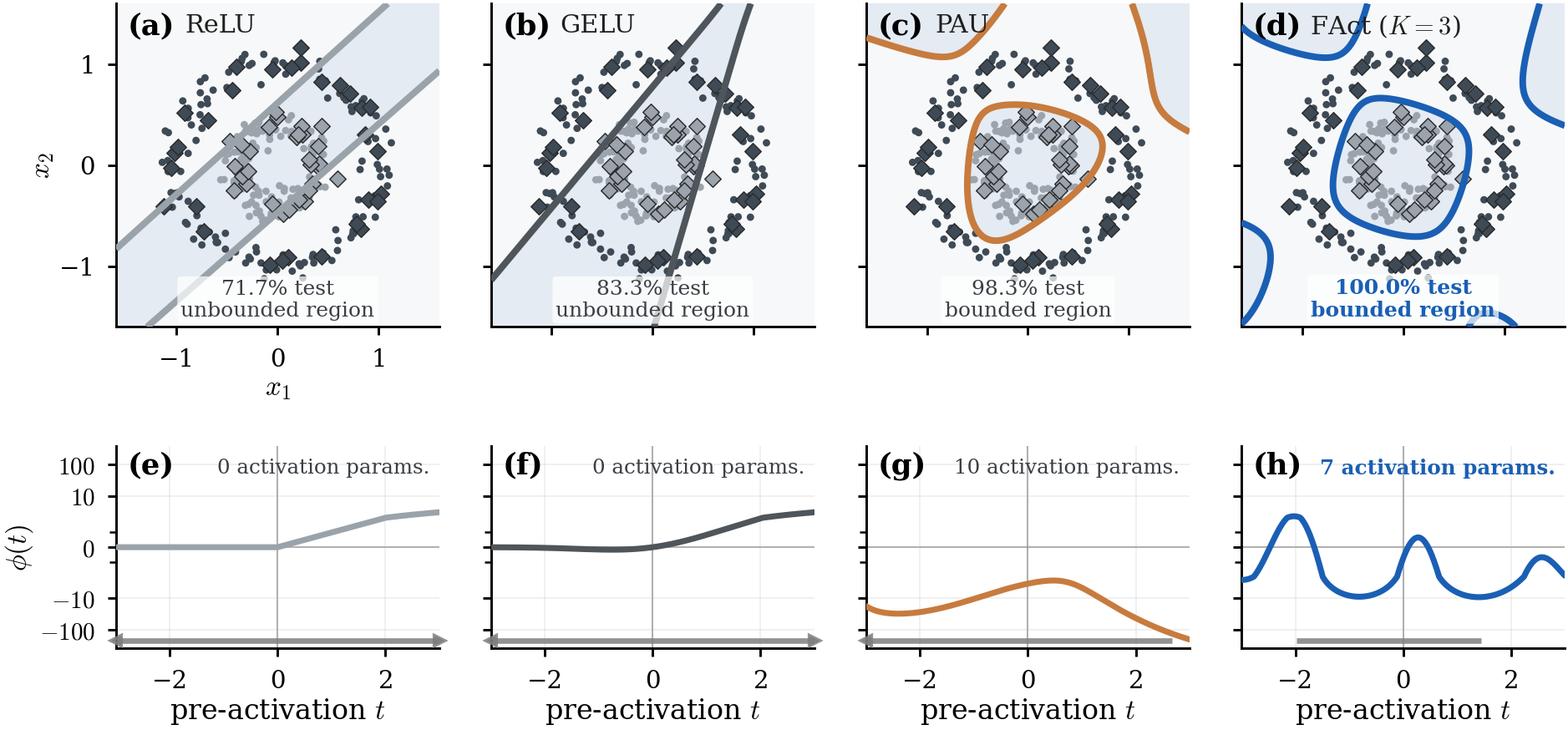
Top: decision regions of a two-hidden-unit network (seed 0) on the concentric circles. Bottom: the corresponding learned activation, on a symmetric-log vertical axis; the grey bar marks the pre-activation range the network actually realizes. ReLU and GELU both settle for an unbounded region and never enclose the inner class at this width. A shared Padé unit (PAU, 10 activation parameters) does produce a bounded region, but only by driving its own output past −200 as its denominator approaches a root. FAct gets the bounded region with 7 activation parameters and stays inside about ±10.
Test accuracy against hidden width, mean ± s.d. over five seeds, with Δ the seed-matched margin of FAct over GELU in percentage points.
Concentric circles, 2 classes, FAct at K = 3 (7 coefficients):
| Hidden units | FAct | GELU | Δ |
|---|---|---|---|
| 1 | 81.3 ± 0.7 | 70.0 ± 15.1 | +11.3† |
| 2 | 100.0 ± 0.0 | 84.3 ± 5.1 | +15.7 |
| 3 | 100.0 ± 0.0 | 99.7 ± 0.7 | +0.3† |
| 4 | 100.0 ± 0.0 | 99.7 ± 0.7 | +0.3† |
| 5 | 100.0 ± 0.0 | 100.0 ± 0.0 | +0.0† |
One-turn spiral, 10 classes, FAct at K = 2 with a learnable ω (6 parameters):
| Hidden units | FAct | GELU | Δ |
|---|---|---|---|
| 1 | 14.3 ± 2.7 | 13.4 ± 1.4 | +0.9† |
| 2 | 20.9 ± 2.7 | 15.9 ± 0.9 | +5.0 |
| 3 | 26.9 ± 2.6 | 19.0 ± 1.1 | +7.9 |
| 4 | 34.4 ± 2.6 | 24.2 ± 0.9 | +10.2 |
| 5 | 45.7 ± 8.2 | 31.4 ± 2.2 | +14.4 |
| 6 | 57.3 ± 3.8 | 33.4 ± 1.5 | +23.9 |
| 7 | 71.3 ± 4.8 | 39.1 ± 3.6 | +32.2 |
| 8 | 81.3 ± 1.5 | 43.4 ± 4.5 | +38.0 |
| 9 | 89.5 ± 2.4 | 48.5 ± 1.4 | +41.0 |
| 10 | 94.0 ± 1.1 | 57.9 ± 4.8 | +36.1 |
† margin short of $p < 0.05$ under a seed-matched paired $t$-test, which on the circles is every width where both activations sit at the ceiling. Both studies use Adam at full batch, learning rate 0.05, five seeds varying only the initialization stream; the circles are scored at the final epoch (500) and the spiral at its best-validation epoch (300 epochs). They are never pooled.
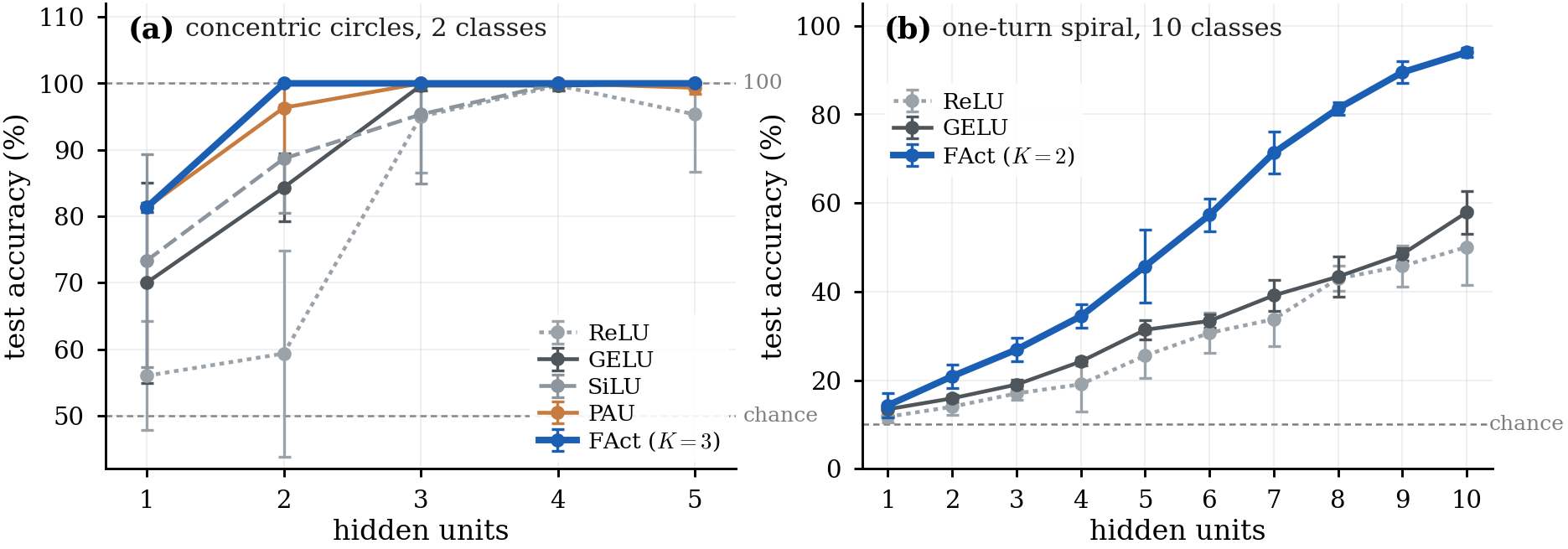
On the circles, FAct is perfect on every seed at two hidden units. GELU needs five. And on the spiral the gap widens with width instead of closing: seven FAct units clear GELU’s ten by 13.4 pp, and six come within 0.6 pp of them. Pooled over the ten widths the seed-matched lead is 21.0 pp ($t = 9.86$, $p = 3.2\times10^{-13}$, 50 pairs). The activation costs six parameters at any width, so the 36.1 pp margin at ten units is bought with 4% more parameters.
These are controlled illustrations at single-digit width, chosen because the capacity question is answerable there. They are not evidence about the ViTs.
The setup, for the record
| Source (ViT-d6) | Target (ViT-d2) | |
|---|---|---|
| Dataset | ImageNet-1K | Fashion-MNIST, CIFAR-10/100, Food-101 |
| Input resolution | 224×224 | 28², 32², 32², 64² |
| Patch size | 16 | 4, 4, 4, 8 |
| Depth | 6 | 2 |
| Embedding dimension | 192 | 64 |
| Attention heads | 6 | 4 |
| MLP ratio (d_ff) | 4 (768) | 4 (256) |
| Parameters, fixed activation | 3,048,232 | 105,098–123,237 |
| Activation parameters | 5, learned jointly | 5, frozen, not updated |
| Training images | 1,271,167 | dataset train split |
| Validation split | 10,000 | 5,000 per dataset |
| Test split | ILSVRC val, 50,000 | dataset test split |
| Seeds | 5 (FAct, GELU), 1 (others) | 6 common, 5 tuned |
| Learning rate / weight decay | 10⁻³ / 0.05 | 10⁻³ / 0.05, or tuned |
Shared by both scales: AdamW, batch size 256, 100 epochs, 5-epoch linear warmup then cosine decay, label smoothing 0.1, dropout 0.1, pad-then-random-crop and horizontal flip (none at test), fp32, best-validation checkpoint evaluated once on test.
What this doesn’t show
Worth being explicit about the edges of the claim.
- Vision Transformers are the primary setting, and that was a deliberate choice. In a convolutional network the same activation is already shared across spatial locations and output channels, so global sharing gets entangled with the spatial weight-sharing structure of the operator. A ViT’s repeated MLP blocks isolate the variable. Other architectures are studied separately.
- At source scale, only FAct and GELU have five seeds. ReLU, LeakyReLU, SiLU and Mish on ImageNet-1K are single runs, marked † in that table, and should be read as such.
- The 30-epoch tuning proxy is imperfect. It occasionally selects a cell that does not hold up at the full budget — ReLU on Fashion-MNIST and CIFAR-100, and LeakyReLU on CIFAR-100, all ended up worse after tuning. Those are the 3 of 44 arms that tuning did not improve.
- One of the eighty transfer margins is not significant after correction.
- The synthetic studies are illustrations, not evidence about models at the scale of the ViT experiments.
Where this leaves things
The thing I find hardest to shrug off is the size of the object being moved. Five numbers, learned inside a 3M-parameter ImageNet model, dropped into a 100K-parameter model on a different dataset with no weights and no adaptation, and they beat every conventional activation there — including after every one of those activations gets its own tuned learning rate and weight decay.
That suggests the nonlinearity is worth treating as a component in its own right: learnable, inspectable, and portable, rather than a fixed design decision made before training starts. Whether the same five numbers survive a jump to convolutional networks, to sequence models, or to a much larger scale is the obvious next question, and not one this work answers.
Citation
The full write-up is Learning and Transferring a Nonlinearity Across Neural Networks, Arun Prakash A, AI4Bharat, IIT Madras. The preprint link will be added here once it is posted; until then, cite it as:
@article{fact2026,
  title   = {Learning and Transferring a Nonlinearity Across Neural Networks},
  author  = {A, Arun Prakash},
  journal = {arXiv preprint},
  year    = {2026}
}