One Learnable Activation, Shared Across the Whole Network — Outperforms Fixed GELU at ImageNet-1K Scale

A quiz before you dive deep

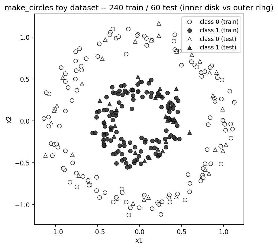
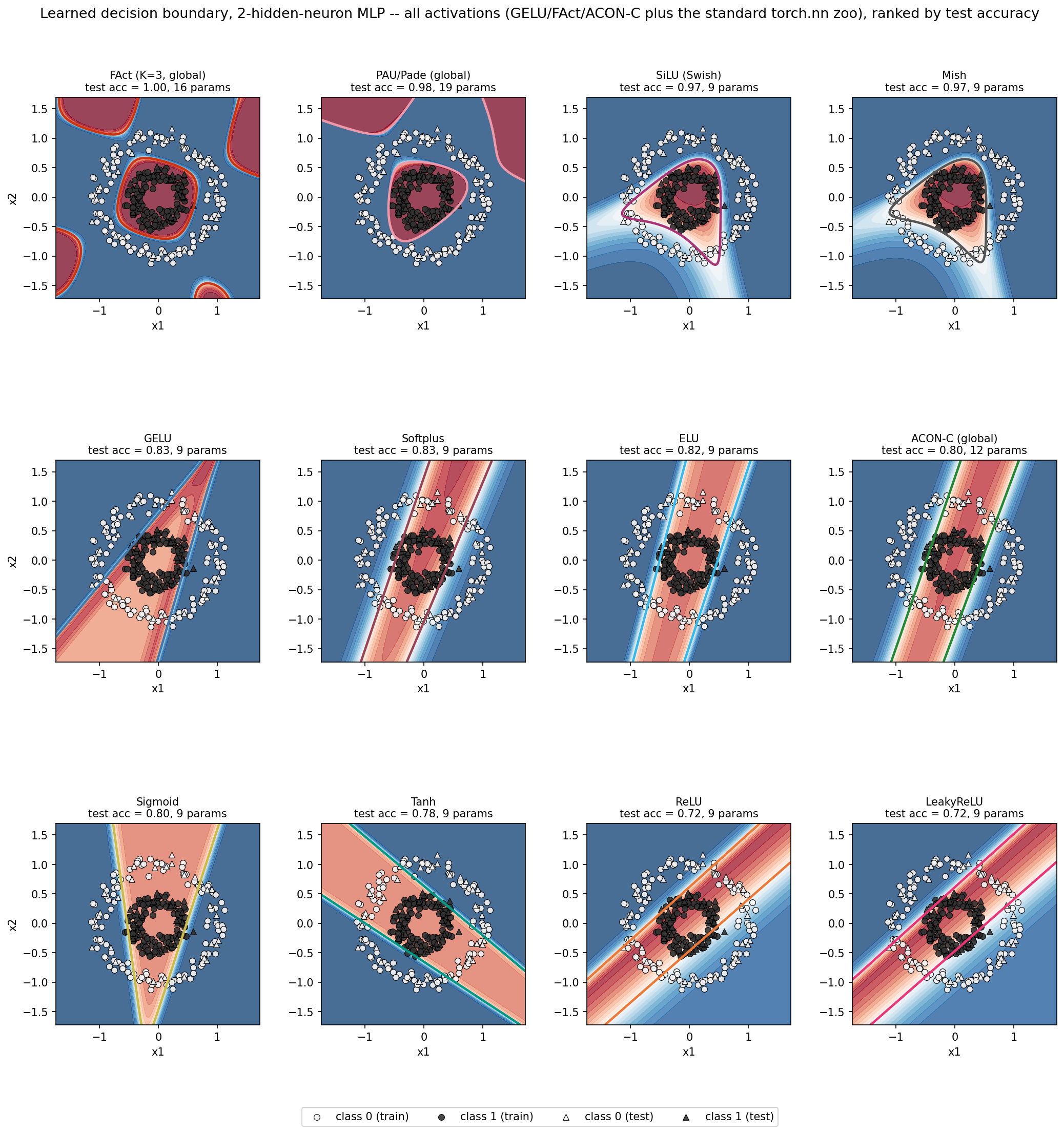
Here’s a circularly separable dataset — an inner disk of one class, surrounded by an outer ring of the other. Suppose you build an MLP with a single hidden layer for it. What is the minimum number of neurons you need in that hidden layer for perfect classification?

Think about it. If you want to confirm your answer, Colah’s blog on neural networks, manifolds and topology is a good place to look.

If you’re convinced the answer is three — congratulations! But…

That is true only if the activation function is fixed.

Learnable activations bring that number down to two. Can every learnable activation do that? Good question — the answer is, obviously, no. Not every learnable activation can pull it off.

Now let’s dive into the study.

While building any neural network, one of the most consequential choices is which activation function to use. There are hundreds of activation functions in the literature, and a handful have become the default — ReLU, GELU, Swish, SiLU, and so on. Either way, we end up fixing the activation function ahead of time, hoping that whatever worked best in someone else’s study will also work best for ours. There have been many attempts to adapt the curve rather than inherit it — but with its shape pre-defined, learning only its curvature. PReLU learns the slope of the negative arm; Swish-$\beta$ learns how sharply the curve bends; ACON generalizes both under a single form. Which family the curve belongs to is still a decision made in advance.

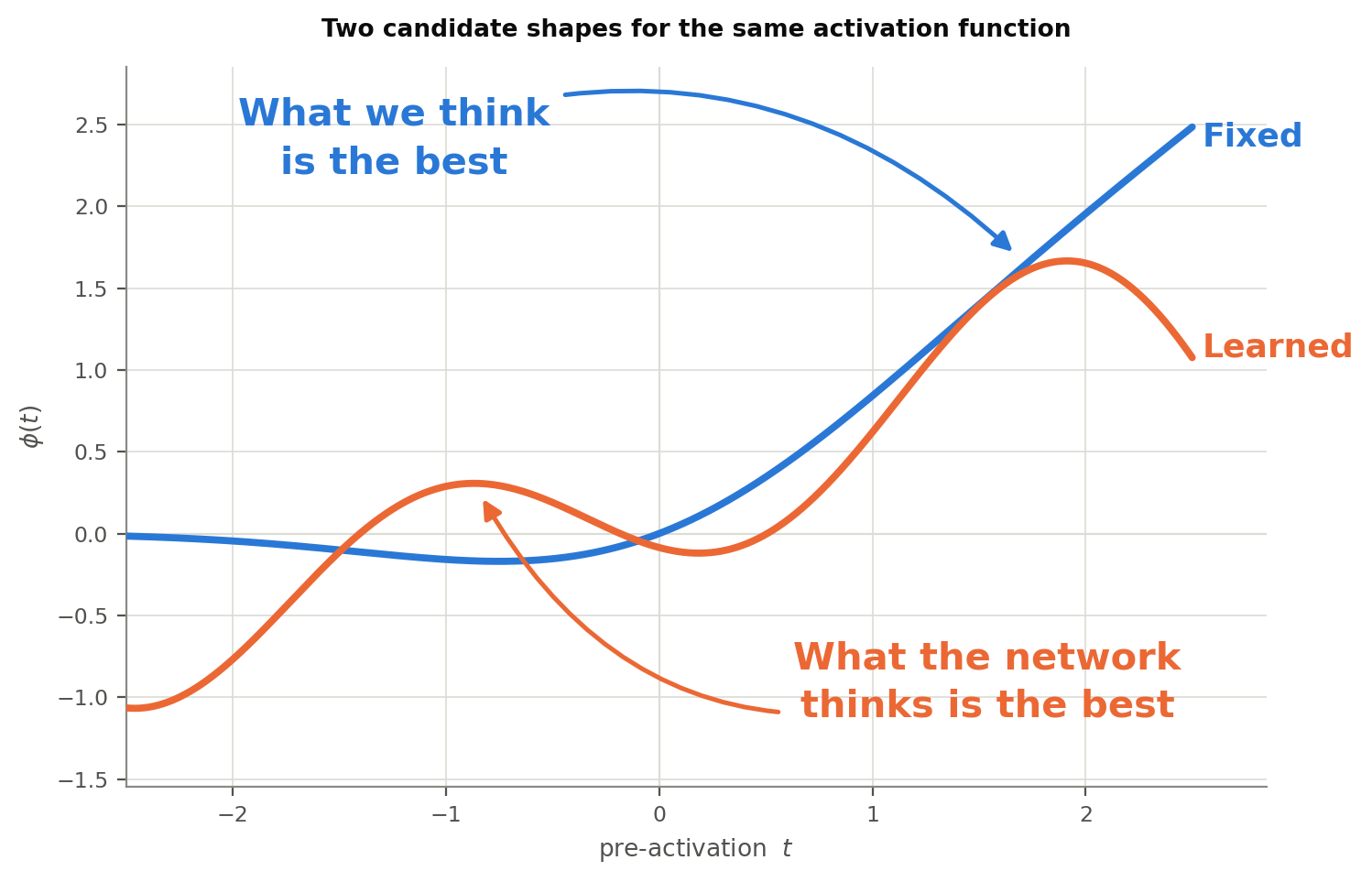
But what if the family isn’t fixed either? What if the whole shape is learned over the interval, instead of a knob on a curve someone else chose? Will it converge faster? Will it deliver better performance?

And there is a third question, the one that makes the global version worth doing rather than just another learnable activation: sharing a single curve across the entire network lets us see what the network wants. Give every channel or every layer its own curve and each is free to specialize, so you get hundreds of answers and no single one — a picture of local preferences, not of the network’s. One curve for the whole network forces every layer to agree on one shape, and the shape they settle on is itself a measurement. Here we study exactly that, and test it at ImageNet scale.

What this study is and isn’t. This isn’t a run at the state of the art. The model here is a small ViT trained on a deliberately plain recipe, and its absolute accuracy is nowhere near the top of the ImageNet-1K leaderboard — that was never the target. The point is narrower and, I’d argue, more interesting: to isolate what happens when a single learnable activation is shared across an entire network, holding everything else fixed, and to measure that difference cleanly enough to trust it. Every comparison below is against a baseline identical in every respect but the activation.

Quick findings:

• It improves performance by +2pp, at 498 of the 500 matched epoch checkpoints — not just at the final one — confirmed across 5 independent seeds.
• It might reshape the network’s landscape geometry: the FFN’s up-projection weight matrices carry a lower spectral norm and a higher stable rank than the fixed activation’s, in every one of the 6 transformer blocks (weight-space evidence, not a direct Hessian measurement — details below).
• Swap the optimizer from AdamW to SGD and the Learnable-over-Fixed gap still holds — at all 100 epochs, with a mean margin even larger than under AdamW (+3.78pt vs +2.57pt). That’s evidence it’s the activation, not the optimizer, doing the work — though on one seed, not five.

The idea

A standard network picks an activation function once and fixes it. This experiment instead gives the network one activation module, shared by reference across every layer, and makes that curve itself a learnable function: it’s a linear combination of five coefficients, initialized to closely approximate the shape of the fixed activation it replaces, and then trained by ordinary backprop exactly like any other weight. The entire network — six transformer blocks, millions of activations computed per forward pass — is bottlenecked through the same five numbers.

Two things make this a clean test rather than a bigger model in disguise:

• It’s shared, not per-layer. One activation object, passed by reference into every block. Five parameters for the whole network, not five per layer.
• It’s tiny. Five extra scalars against three million weights — a parameter increase small enough to round to zero.

If this helps, the interesting claim isn’t “bigger activation modules are good” — it’s that what shape the nonlinearity takes is doing more work than we usually give it credit for, and handing that shape to gradient descent is cheap.

Related work

Learning the activation instead of fixing it is an old idea, reinvented independently in several communities. What none of it shows — not to my knowledge — is a single activation shared by the entire network that outperforms either the fixed default or the learnable versions shared per channel or per layer. The map below is largely a map of sharing strategies: almost everything in it is shared across channels or across layers, and that is what makes the activation budget grow with the model — dozens to tens of thousands of extra parameters on the small ViT used here. Per site the counts are modest: one number for PReLU, three for ACON, ten for PAU. But they are per site. Ours is five, and five is also the total.

	What’s learned	Shared across	Activation params	IN-1K
ReLU / GELU	nothing	—	0	✓
PReLU, Swish-$\beta$, ACON	a knob on a known shape	channel	1–3 / channel	✓
APL	shape, from hinges	neuron	$2S$ / neuron
PAU, rational nets	whole shape, rational basis	layer	~10 / layer	✓
DeepLABNet	whole shape, RBF basis	unit	per unit
KAN, F-KAN, KAF	whole shape, spline / Fourier	every edge	scales with weight count	✓
SIREN	nothing — $\omega_0$ is a hyperparameter	—	0
STAF	amplitude, frequency, phase	neuron	3 / harmonic / neuron
GAAF, LAAF	a scale inside a fixed shape	whole network / layer	1 total
This study	whole shape, Fourier basis	whole network	5 total	✓

IN-1K = reports ImageNet-1K results; blank means not to my knowledge.

How this work differs

We’d like to emphasize the same gap once more, because it is the whole point: everything that learns the whole shape pays for it per layer, per unit or per edge — the activation budget grows with the network.

Put that on the model in this experiment — a depth-6 ViT-Ti/16 with 768 hidden units per block, so 4,608 activation sites. ACON-C learns three channel-wise numbers $(p_1, p_2, \beta)$ at each one: 13,824 extra parameters. A per-edge basis like KAN’s would put a small learned function on each of the 1.77M FFN weights. The activation here is five numbers — and it is still five numbers at ViT-L, because it does not scale with anything.

The only entry in the table that shares network-wide, GAAF, learns a single scale inside a shape that never changes — and has never been run on vision at all. What we designed is the conjunction:

• the whole shape, learned — not a knob on a known one
• shared by every layer — five numbers for the entire model
• inside a transformer
• at ImageNet-1K scale
• against a matched baseline over multiple seeds
• and, as a consequence of the sharing, a single curve to look at

Why Fourier Approximation of the activation

First, is a basis even needed? Why not just use ACON globally, which has only three parameters?

ACON is the strongest member of the knob-on-a-known-shape family: it smoothly interpolates between $\max(p_1 t,\, p_2 t)$ and a linear map, recovering ReLU, Leaky ReLU, PReLU and Swish as special cases, for three numbers. So we shared those three numbers globally, exactly the way ours are shared, under a byte-identical recipe. We called it at 50 epochs: ahead of fixed GELU at only 37 of them, by +0.5 pt on average, and inside GELU’s own five-seed noise band at roughly two thirds of them. Run ACON the way its paper prescribes instead — per channel, per layer, 13,824 parameters — and on this model it falls below the fixed baseline.

Activation	Params	$\Delta$ vs GELU, ep 1–25	$\Delta$ vs GELU, ep 26–50	Ahead of GELU	Inside GELU’s $\pm 2\sigma$
Fourier, shared	5 total	+2.64 pt	+2.32 pt	100 / 100 ep	0 / 50 ep
ACON-global	3 total	+0.86 pt	+0.15 pt	37 / 50 ep	32 / 50 ep
ACON, per channel per layer	13,824	−1.18 pt	−2.53 pt	1 / 42 ep	11 / 42 ep

Seed 1, identical recipe. Each window is cut to the run’s own depth — the per-layer leg stopped at 42, ACON-global at 50, the Fourier leg ran all 100. $\pm 2\sigma$ is GELU’s own five-seed spread at each epoch: a row sitting inside it is not distinguishable from changing the random seed.

ACON-global buys almost nothing. Three knobs on a fixed shape are not a shape. $p_1$ and $p_2$ set two slopes and $\beta$ sets how sharply they meet; whatever those numbers do, the curve remains two lines joined by a knee. One curve serving an entire network appears to need something else: the freedom to change shape across the interval, smoothly. That is a property of the basis, not of the parameter count.

The Fourier basis has that property. $\lbrace 1,\, \cos kt,\, \sin kt \rbrace$ is complete in $L^2[-\pi, \pi]$, so the family can represent any square-integrable shape on the interval, and every truncation of it is infinitely differentiable. The completeness belongs to the family, not to the five numbers — $K$ sets how much of the basis is actually in play, and $K = 2$ is a deliberate stop at low frequencies.

The shared curve is a truncated Fourier series in the pre-activation $t$:

\[\varphi(t) \;=\; a_0 \;+\; \sum_{k=1}^{K} \left[\, a_k \cos(k\omega t) \;+\; b_k \sin(k\omega t) \,\right]\]

with $K = 2$ and $\omega = 1$, so the learnable set is $\lbrace a_0, a_1, a_2, b_1, b_2 \rbrace$ — the five numbers. They are not fitted or randomly initialized: GELU’s Fourier coefficients on $[-\pi, \pi]$ are computed by numerically integrating the Euler formulas, giving $a_0 = 0.7061$, $a = [-0.7049,\ 0.0261]$, $b = [1.0000,\ -0.5000]$. Training starts from a curve that already is the activation it replaces, and every later shape is a departure the gradient chose to make.

Why a Fourier series. Five numbers serving an entire network have to be well-behaved, and that is mostly a property of the basis:

• Bounded, nothing to divide by — $|\varphi| \le 2.43$ at init, since $\sin$ and $\cos$ live in $[-1, 1]$. Rational bases carry a denominator that can approach zero (PAU needs a “safe” variant to fence off the poles); polynomial bases have the opposite failure and diverge as $|t|$ grows.
• No vanishing gradient in the tails — $|\varphi’| \le 2.23$ at init, and being periodic it does not decay with $|t|$ the way sigmoid and tanh saturate. A large pre-activation isn’t a dead one.
• The basis never amplifies gradient to the coefficients — $\partial\varphi/\partial a_k = \cos(kt)$ and $\partial\varphi/\partial b_k = \sin(kt)$, in $[-1, 1]$ for any input at all. That bound matters more here than it would per-layer: these five accumulate gradient from every activation site in the network, every step.
• Orthogonal on $[-\pi, \pi]$ — the five parameters move along near-independent directions. Monomial bases are ill-conditioned by comparison; splines need a grid range to tune. There’s no grid here.
• Graceful truncation — the coefficients of a smooth reference decay fast, which is why $K=2$ already carries the shape: at init the second harmonic’s amplitude is 0.50 against the first’s 1.22.

It holds up in practice too: independent seeds land within 0.02 of each other.

That leaves two things under test — whether the global version survives real scale (sharing is where it’s most likely to break: one curve now serves every layer, and transformer layers aren’t doing the same job), and whether it holds under a controlled measurement (five matched seeds, bit-identical init, all 500 epoch checkpoints, a paired test).

Other bases are available, and two were tried. Padé — the real PAU, shared globally the same way — turned out to be a genuine contest: wherever it trains to completion, it holds its own against the Fourier version on accuracy. What separates them is stability and cost. Under mixed precision it diverged on the harder dataset, on every seed, where the Fourier runs never did. Forcing full precision fixes that, but makes it slow enough that carrying it to ImageNet was no longer affordable — that run was abandoned early. Chebyshev failed the way the polynomial bullet above predicts: pre-activations ran away and the forward pass went to NaN.

So the finding isn’t that the alternatives fail. It’s that Fourier matches the best of them on accuracy while staying stable in half precision and cheap enough to run at scale, on fewer parameters.

The setup

Model	depth-6 ViT-Ti/16 (patch 16, $224\times224$, $d_{\text{model}}=192$, 6 heads)
Dataset	ImageNet-1K — 1.27M train / 10K val / 50K official test
Optimizer	AdamW, lr 1e-3, weight decay 0.05, cosine schedule, 5-epoch warmup
Epochs	100, both variants, 5 matched seeds
Augmentation	RandomResizedCrop + flip only — no mixup, no RandAug
Fixed	the standard activation, no learnable parameters
Learnable	one shared activation, +5 parameters, network-wide
Params	3,048,232 (Fixed) vs. 3,048,237 (Learnable)

Everything else — architecture, data pipeline, schedule, seeds — is held identical. Initialization was checked bit-for-bit equal between the two variants at matched seed, so the activation is the only thing that differs.

Results

Fixed: 62.45% top-1. Learnable: 64.38% top-1. A +1.93 point gain, for five extra numbers, holding at 498 of the 500 matched epoch checkpoints, across five independent seeds.

Test top-1 (official 50K val)	Fixed	Learnable	$\Delta$
seed 1	62.50%	65.12%	+2.62
seed 2	62.56%	64.33%	+1.77
seed 3	62.49%	63.96%	+1.47
seed 4	62.23%	64.24%	+2.01
seed 5	62.49%	64.27%	+1.78
mean ± s.d.	62.45 ± 0.13%	64.38 ± 0.44%	+1.93 ± 0.43

Paired across all five seeds: $t(4) = 10.02$, $p = 0.00056$. Best-validation accuracy tells the same story: 64.98% → 67.03%, +2.06 ± 0.54 pt, $t(4) = 8.45$, $p = 0.00108$.

How many epochs does it save?

Another way to read the same gain: how many epochs each variant needs to first reach a given validation accuracy, meaned over the five seeds.

val-acc threshold	Fixed	Learnable	epochs saved
50%	27.6 ± 1.0 (5/5)	22.2 ± 1.7 (5/5)	5.4
55%	49.6 ± 1.6 (5/5)	42.4 ± 2.3 (5/5)	7.2
60%	70.8 ± 1.3 (5/5)	61.4 ± 1.9 (5/5)	9.4
65%	98.5 ± 1.5 (2/5)	82.8 ± 1.6 (5/5)	16.5 (n=2)

The bracketed fraction is how many of the five seeds cleared that threshold at all inside 100 epochs. The saving widens as the bar rises — 5 epochs at 50%, 9 at 60% — and by 65% it stops being a saving and turns into a difference in kind: all five Learnable runs get there, with a schedule to spare, while only two of five Fixed runs manage it at all, and those two only at epochs 97 and 100. The other three finish at 64.8%, 64.9% and 64.8%, short of the line. That’s why the last row is an n=2 comparison and the weakest of the four.

It’s not just a better final number — it’s ahead the entire time

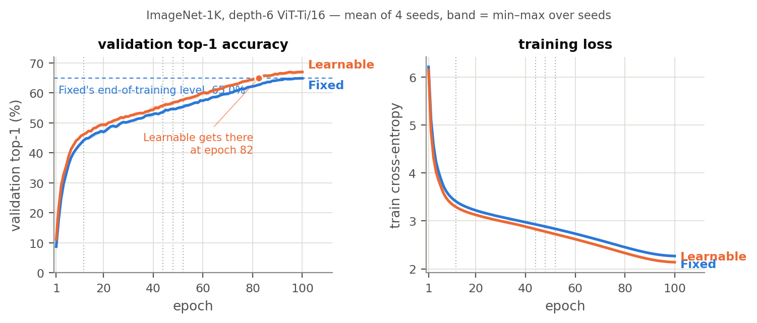
Learnable tracks above Fixed from very early in training and stays there, with two brief exceptions covered in the next section. It reaches Fixed’s entire 100-epoch validation accuracy at epoch 83 on average across the five seeds (individually: 80, 82, 87, 81, 84) — the same final quality, with ~17% of the training budget still on the table.

The gap is negative at just 2 of 500 checkpoints — and recovers immediately

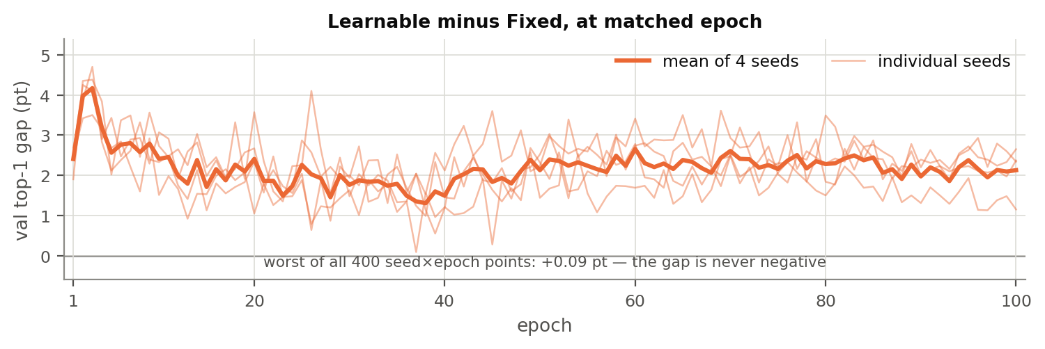
Five seeds × 100 epochs = 500 matched comparison points. With four seeds this gap had never gone negative; the fifth seed breaks that streak, barely — seed 5 dips to −0.15 pt at epoch 23 and −0.11 pt at epoch 32, both early/mid training, both gone by the next logged epoch. Every other point, 498 of 500, favors Learnable. The gap is noisy epoch to epoch (a 10K validation split will do that), and at this sample size two brief dips read as noise, not a real regression.

What did five numbers learn to do?

The three seeds below had their weights checkpointed every epoch; the fourth and fifth seeds above confirm the accuracy gain but weren’t checkpointed at that resolution, so this section and the next two stay 3-seed.

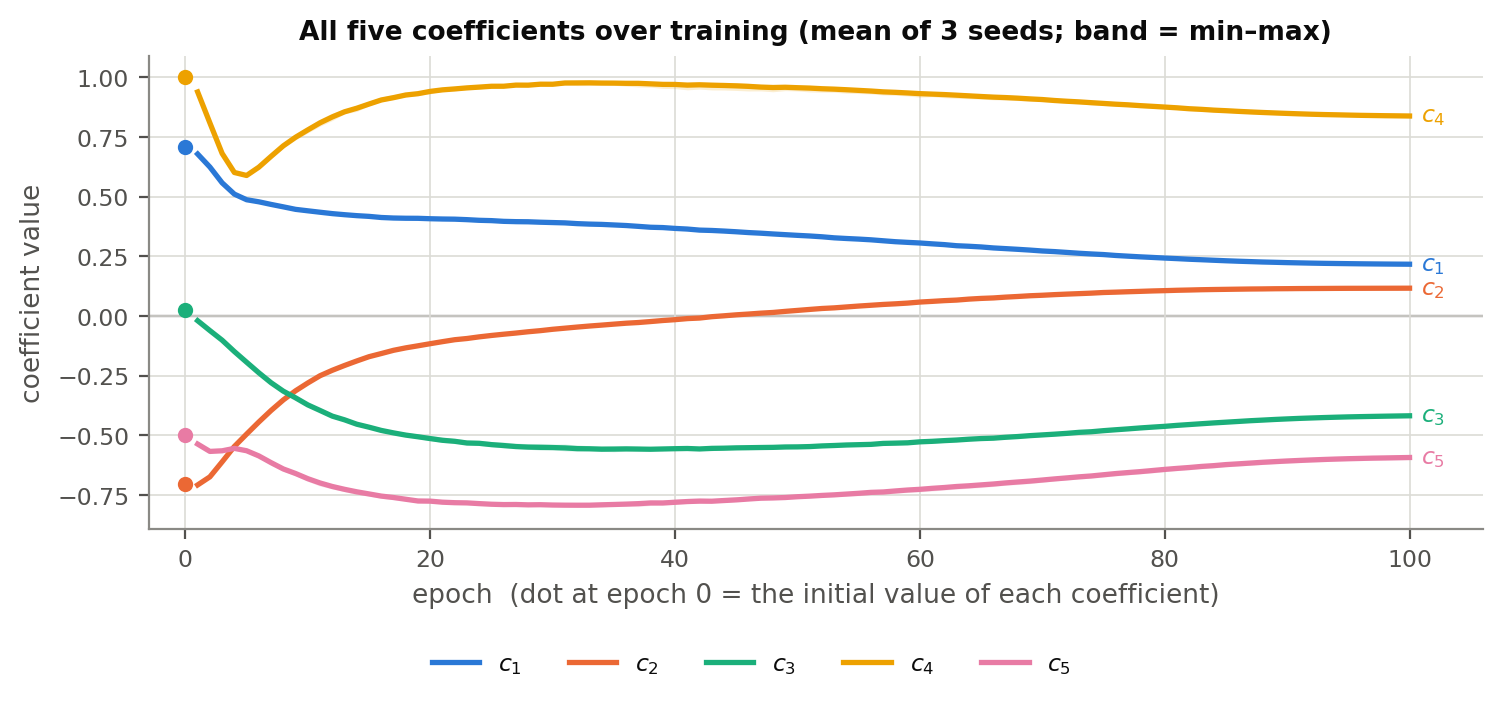
The coefficients move a lot early — a sharp swing in the first ~5 epochs, then a slower drift for the rest of training — and they land in essentially the same place regardless of seed. The largest disagreement between any two seeds, in any of the five coefficients, at any epoch, is 0.033. Three independently-initialized runs converge to the same curve. That’s not noise; that’s the training problem pulling on the activation the same way every time.

That early swing is also where the accuracy gain is widest. Averaged over the five seeds, Learnable’s lead over Fixed is +3.15pt across epochs 1–5 — peaking at +3.95pt at epoch 3 — against +2.01pt over epochs 21–100, once the coefficients have largely settled. The advantage is at its largest while the activation is still visibly changing shape, then narrows to a smaller margin that holds steady for the rest of training. Most of what the five parameters are worth, they appear to be worth early.

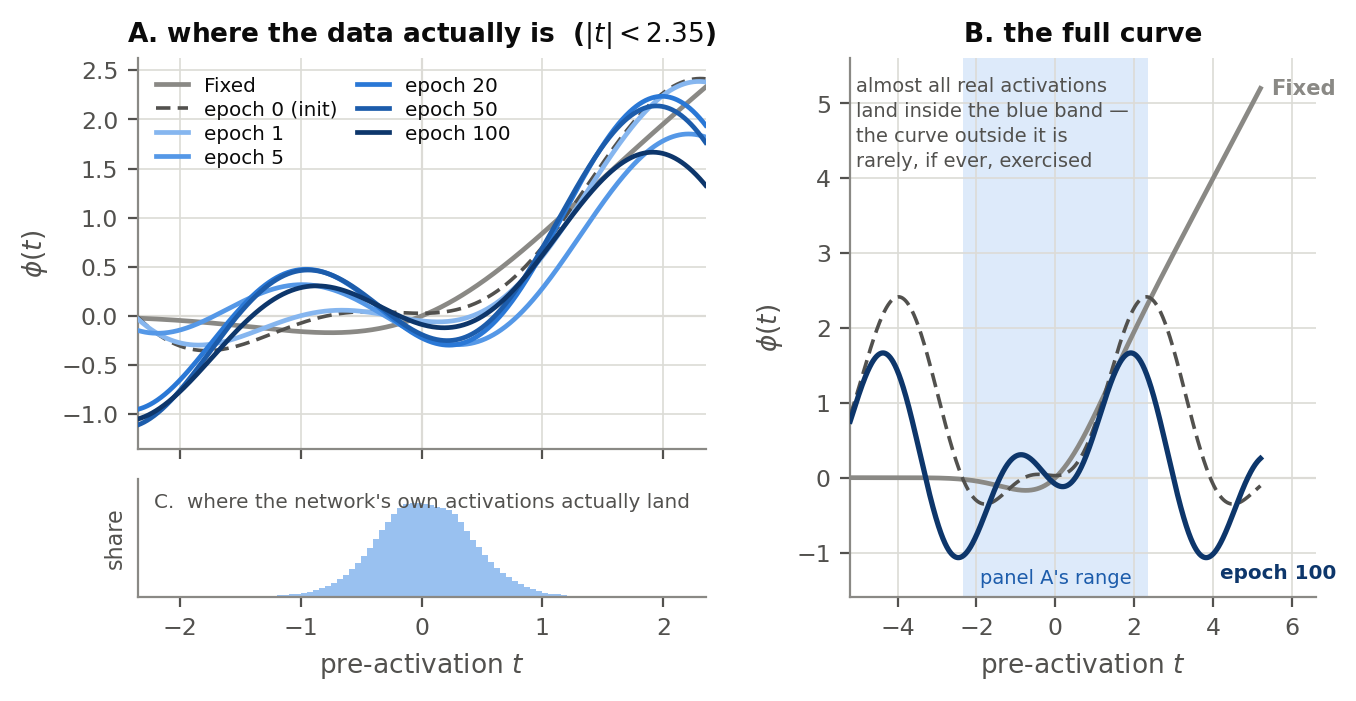
Panel A is the part that matters: zoomed to the range where the network’s actual pre-activations live (panel C shows that distribution directly), the learned curve settles into something with a bit more curvature than the fixed activation it started from — not a wild departure, but a real, reproducible reshaping of the function every unit in the network is computing.

Questioning common assumptions about the shape of the activation

• Monotonicity isn’t load-bearing here. Local max at $t \approx -0.87$, local min at $t \approx +0.19$ — two real, seed-independent inflections sitting right where the network’s own pre-activations actually live (mean $|t| \approx 0.33$, 99% within 1.21), not off in some rarely-visited tail.

• The slope at zero didn’t shrink toward the fixed activation’s — it crossed to the other side and stayed there. +0.5 (fixed) → −0.35 (learned, epoch 100), landing within 0.02 of each other across all three seeds (−0.352, −0.356, −0.339).

• The one feature credited with the fixed activation’s edge over ReLU relocated instead of disappearing. Its dip sat at $t \approx -0.75$; in the learned curve that region is lifted to a small positive bump, and the dip reappears just past zero, at $t \approx +0.19$.

• A shape this specific, reproduced this exactly, argues against “any smooth default will do.” Three independent seeds, under active weight decay, land on the same non-monotonic, sign-flipped curve.

• Getting the far field “wrong” costs next to nothing, because the far field is nearly empty. The curves diverge sharply past $|t| \approx 2$, but almost no real pre-activation ever lands there (0.013% outside $\pm\pi$, none outside $\pm 2\pi$).

Does FAct Reshape the Spectral Geometry of the Network?

A direct answer would need the Hessian of the loss — we don’t have that here. What we do have is the singular-value spectrum of every FFN weight matrix (fc1, the up-projection, and fc2, the down-projection) in all 6 transformer blocks, at 10 checkpoints across training, for both variants (seed 1). Two standard scalar summaries of that spectrum are a reasonable weight-space proxy for “how extreme a map this layer computes”: the spectral norm (the top singular value — an upper bound on how much the layer can stretch its input in any direction, i.e. a Lipschitz-constant proxy) and the stable rank ($\lVert W\rVert_F^2 / \lVert W\rVert_2^2$ — how spread the weight’s energy is across directions, versus concentrated in one).

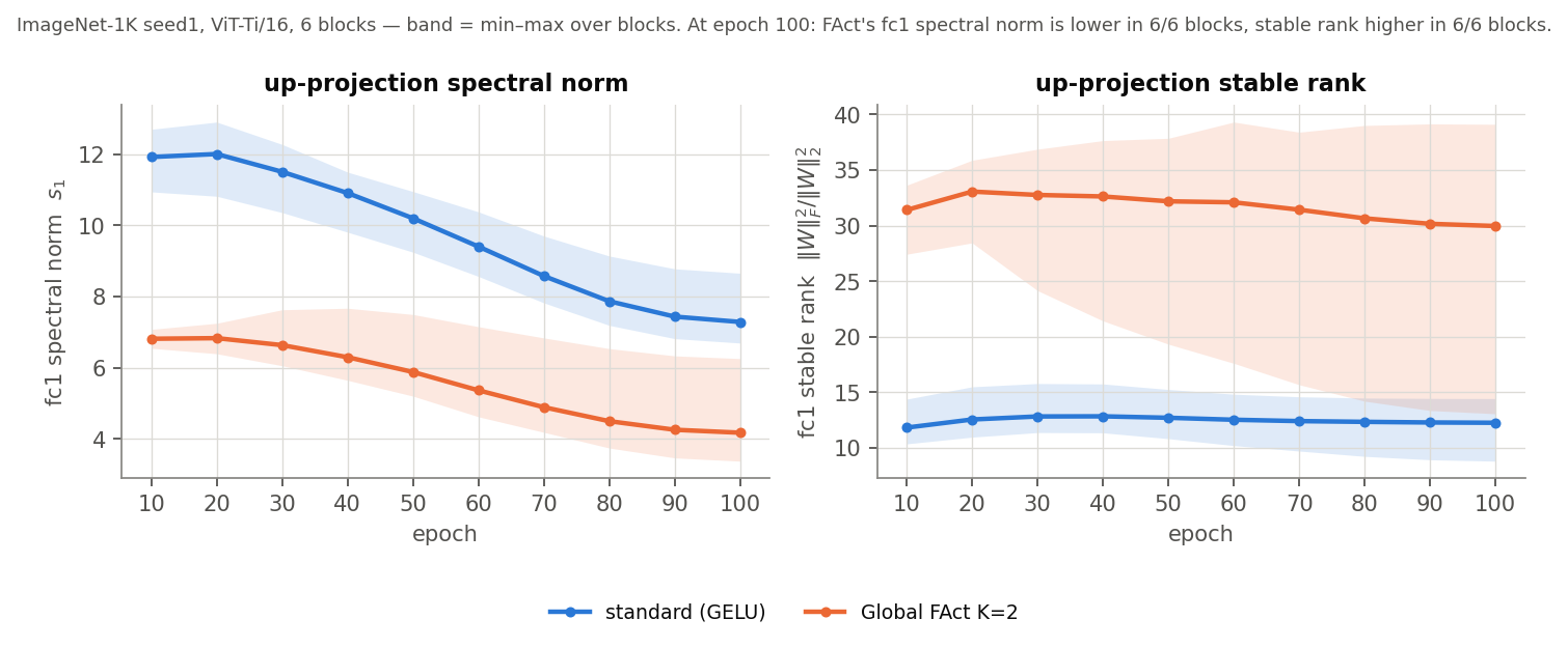
For the up-projection (fc1), the pattern is completely consistent: at every checkpointed epoch, in every one of the 6 blocks, Learnable’s weight matrix has both a lower spectral norm and a higher stable rank than Fixed’s — at epoch 100, roughly half the spectral norm and 2-3× the stable rank in most blocks. That’s a less extreme, less anisotropic linear map at every stage of training, not just at convergence. The down-projection (fc2) doesn’t show the same clean separation — it’s mixed across blocks, sometimes favoring one variant and sometimes the other — so this is presented as fc1-specific evidence, not a network-wide claim, and it’s weight-space geometry rather than a curvature measurement of the loss itself.

Is it the activation, or just AdamW?

Everything above uses AdamW. The obvious challenge: maybe the +2pp gain is an AdamW artifact — some interaction between the learnable coefficients and Adam’s per-parameter adaptive updates — rather than a property of the activation itself. If that were true, swapping in a different optimizer should shrink or erase the gap. So the same seed-1 comparison was re-run under plain SGD (lr=0.05, momentum 0.9, Nesterov) instead, for both variants. Both legs have now finished all 100 epochs — an earlier version of this section reported them mid-flight, over the first 31 epochs; what follows is the completed comparison.

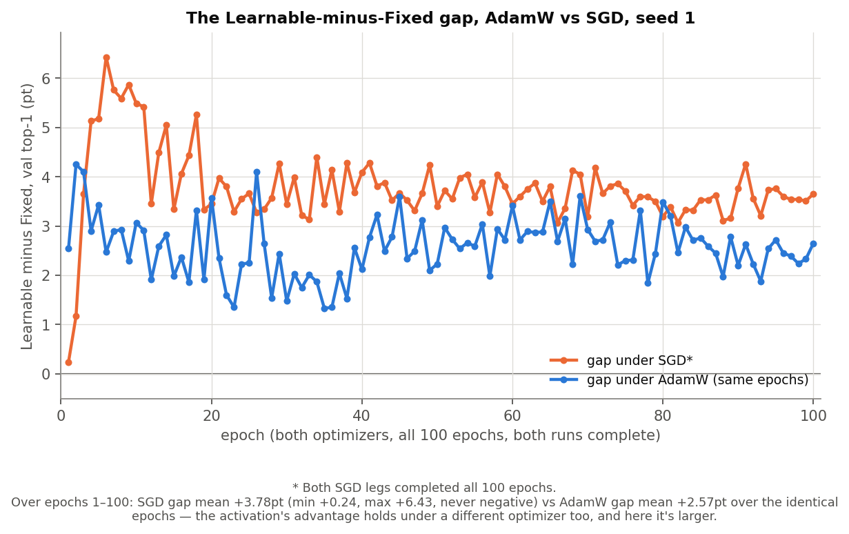
The gap survives the optimizer swap, and it’s larger, not smaller. Across all 100 epochs, Learnable beats Fixed at every single epoch under SGD too — mean gap +3.78pt (min +0.24, max +6.43, never negative), against a +2.57pt mean for AdamW over the identical epochs. Two optimizers with unrelated update rules, different learning rates, different implicit biases — same qualitative result, same direction, same “never negative” pattern the AdamW comparison showed on 4 of its 5 seeds. That’s the actual validation this section is after: the advantage isn’t riding on AdamW’s adaptive moments, it’s coming from the shape of the nonlinearity itself. The partial-run numbers held up: the mean SGD gap settled from +4.09pt over the first 31 epochs to +3.78pt over all 100, still comfortably above AdamW’s.

Under SGD the crossover is earlier, too. Learnable reaches Fixed’s entire 100-epoch best validation accuracy at epoch 67 — a third of the schedule left over, against the epoch-83 crossover the AdamW runs showed.

All four runs on one pair of axes — both variants, both optimizers, the full 100 epochs:

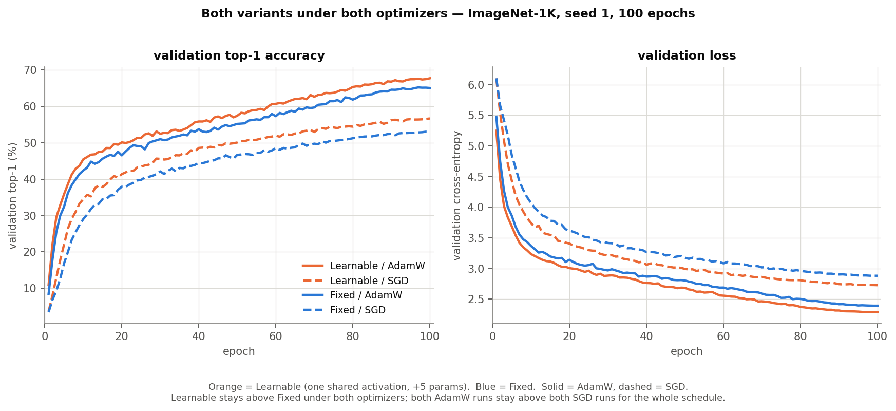
Within each optimizer, Learnable sits above Fixed for the whole run — solid above solid, dashed above dashed. Between optimizers, the two AdamW curves sit well above the two SGD ones throughout.

However, SGD converged more slowly than AdamW in absolute terms for both variants under these particular hyperparameters, and it never caught up. Final validation accuracy: Fixed 53.01% (SGD) vs 65.18% (AdamW), Learnable 56.65% (SGD) vs 67.68% (AdamW). That’s a statement about optimizer speed, not about the activation, and it’s orthogonal to the gap result above — a slower-converging optimizer can still show a larger relative advantage for Learnable at matched epochs. So the question this section used to leave open now has both halves answered: the Learnable-over-Fixed gap holds all the way to epoch 100, and SGD’s absolute level does not close on AdamW’s. These are single-seed results, unlike the five-seed AdamW comparison above, so they carry correspondingly less weight.

Limitations

The accuracy is bought with wall-clock time. A fixed activation like GELU is one cheap elementwise op. The learnable one is a truncated Fourier series, so every activation site evaluates four transcendental functions — two sines and two cosines — instead. Standard FLOP counters miss this entirely: they tally matmuls and convolutions, so both variants score an identical 1.283 GFLOPs forward and 3.791 GFLOPs forward+backward per image. The cost is real nonetheless, and the reason is worth stating plainly:

sin and cos execute on the GPU’s special-function units, which have far less throughput than the tensor cores doing the matmuls.

The activation isn’t competing for the same hardware the rest of the network runs on — it’s queued for a much narrower lane.

Worth adding that this is an implementation cost, not a mathematical one, and that what’s measured above is the naive implementation. It builds a $(\text{batch} \times \text{features} \times K)$ tensor of angles and calls cos and sin across all of it, so $K=2$ really does evaluate four transcendentals per activation and write three intermediates out to memory. Neither is necessary. The double-angle identities give $\cos 2t$ and $\sin 2t$ from a single sin/cos pair almost for free, and a fused kernel could keep the whole series in registers instead of round-tripping through memory.

Attention was in this exact position once. The mathematics never changed; an implementation that respected the memory hierarchy turned it from the thing you budget around into the thing you stop thinking about. There’s no FlashAttention for learnable activations yet — we’d like there to be. 🙂

Update (2026-08-16): we went and wrote that fused kernel — a hand-written CUDA forward and analytic backward for the $K=2$ series ($\phi(t) = a_0 + a_1 \cos(wt) + b_1 \sin(wt) + a_2 \cos(2wt) + b_2 \sin(2wt)$), one sincos() call per harmonic instead of separate cos/sin ops, the whole forward (and backward) fused into a single elementwise pass, with a block-level reduction before the coefficient gradients’ atomics. Benchmarked forward+backward against both GELU and the naive PyTorch reference above, on an NVIDIA L4 (23GB) and an H200 NVL (143GB):

GPU	shape (B, N, d_ff)	GELU	naive FAct	CUDA-kernel FAct	kernel vs. naive	kernel vs. GELU
L4	(64, 197, 384)	0.88 ms	6.74 ms	4.16 ms	1.62x faster	4.71x slower
L4	(256, 197, 384)	1.66 ms	28.91 ms	16.47 ms	1.76x faster	9.94x slower
L4	(256, 197, 1536)	6.64 ms	114.83 ms	65.73 ms	1.75x faster	9.90x slower
H200	(64, 197, 384)	0.70 ms	3.13 ms	2.00 ms	1.56x faster	2.86x slower
H200	(256, 197, 384)	1.07 ms	9.05 ms	1.86 ms	4.87x faster	1.74x slower
H200	(256, 197, 1536)	1.30 ms	34.62 ms	7.13 ms	4.86x faster	5.49x slower

Progress, not parity. The kernel is 1.6–4.9x faster than the PyTorch-composed reference it replaces — on the H200, at the two larger shapes, it gets within 2x of GELU — but across the shapes tried it’s still 1.7–9.9x slower than GELU, not on par with it yet. Correctness (forward, grad_input, and every coefficient gradient) was checked against the reference to double-precision tolerance and passed gradcheck, so the speedup isn’t coming from cut corners.

The bigger surprise was memory, not speed. The naive reference materialises a $(\text{batch} \times \text{tokens} \times \text{features} \times K)$ tensor of angles, then separate cos and sin tensors of that same shape, and autograd keeps all of it alive for backward. The kernel’s backward instead recomputes sin/cos per-thread from the raw input, so it only ever needs to keep the input itself (plus the five scalar coefficients) resident:

shape (B, N, d_ff)	naive FAct (MB)	CUDA-kernel FAct (MB)	reduction
(64, 197, 384)	221.6	18.5	12.0x
(256, 197, 384)	888.0	74.0	12.0x
(256, 197, 1536)	3552.0	296.0	12.0x

A flat 12x at every shape, on an A100, an L4, and an H200 alike — which makes sense, since the multiple is fixed by how many (batch × tokens × features × K)-sized tensors the naive path keeps around, not by anything architecture-specific. This is arguably the more practically important number of the two: it’s the difference between a given batch size or d_ff width fitting on the GPU at all and hitting an OOM outright, which the naive reference did mid-benchmark on a contended GPU while the kernel kept running.

There’s headroom left — parameter-gradient reduction still round-trips grad_output and input through global memory rather than fusing with the forward pass, and $K=2$ is the only harmonic count this kernel hand-unrolls. Still no FlashAttention moment. But it’s a first step toward one.

Appendix

A. How the prior work reports its results

Since this study leans on seeds, per-epoch tracking and wall-clock honesty, it seems only fair to ask how the work in the table above reports its results. Compiled in August 2026.

Method	Code	Seeds	Wall-clock	Gain shown over training
APL	✓ Caffe model/solver files	55 runs, mean ± std	✗	✗ final numbers only
PAU	✓ (superseded; demos are MNIST/F-MNIST)	5 seeds ± — but not on ImageNet	✗	✓ curves, incl. ImageNet
Rational nets	✓	✗	✗	✓ validation-loss curves
ACON	✓ full ImageNet pipeline + weights	✗	FLOPs/params only	one appendix figure
KAN	✓ actively maintained	3 seeds, some experiments	grid-size scaling only	mixed
GAAF / LAAF	✓ but a Burgers PINN demo, TF 1.14	✗ GAAF; 3 trials on LAAF’s CIFAR/SVHN	✗	✓ loss vs epoch
F-KAN	✗	± given, n never stated	✗	✓ convergence curves
KAF	“will release” post-review	✗	GPT-2 only, not vision	✗ ImageNet = final table
STAF	project page, no repo found	✗	appendix mention	✓ PSNR trajectories
SIREN	✓	✗	one anecdote	—
DeepLABNet	✗ none found	✗	✗	—

Multiple seeds are rare, and rarest exactly where they matter. PAU is explicit about it: “In all experiments except for ImageNet, we report the mean of 5 runs initialized with different seeds.” They ran five seeds everywhere and dropped the protocol at ImageNet scale — understandably, since that’s where the compute hurts. ACON and KAF are single-run too. Every ImageNet-scale learnable-activation result I checked is a single run.

Wall-clock overhead is essentially unreported — 0 of 11 give a training-time comparison against their own baseline. KAF’s GPT-2 timing is the only real number and it’s off-task. That’s a conspicuous gap for a family of methods whose defining feature is replacing a cheap elementwise op with something expensive: PAU divides, KAN evaluates splines, the Fourier line calls transcendentals. The 2.2× above is not a flattering number, but it appears to be one of the few published at all.

Code release is common but shallow. Seven of eleven ship something, yet most is the activation module rather than a pipeline; ACON is the only one with training code and pretrained weights for ImageNet.

B. The same question on small and medium datasets

The ImageNet run above is one architecture. This is the same question asked four more times, on a convolutional backbone instead of a transformer, with an extra control that ImageNet never got: arms that share globally but learn only one number.

The backbone is a MetaFormer-style mixer at a fixed ~100K-parameter budget — LinearConv → shared channel-MLP → pool, twice, then GAP and a two-layer head — and every activation site in it is served by one module passed by reference, exactly as in the ViT. Four arms, five seeds each:

Arm	What is learnable	Extra params
standard	nothing (GELU)	0
prelu_global	one negative slope	1
swish_global	one $\beta$ in $x\cdot\sigma(\beta x)$	1
fact_k2_global	the whole shape	5

Test accuracy, mean ± std over 5 seeds, with a paired two-sided $t$-test against standard (df = 4, so $|t| > 2.776$ is $p < 0.05$):

Dataset	Epochs	standard	prelu_global	swish_global	fact_k2_global
Fashion-MNIST	30	87.22 ± 0.49	87.68 ± 0.30 +0.45 ($t=1.53$)	87.14 ± 0.95 −0.08 ($t=-0.17$)	89.00 ± 0.44 +1.78 ($t=7.34$)
CIFAR-10	40	66.98 ± 0.49	68.71 ± 0.27 +1.73 ($t=8.05$)	66.43 ± 0.45 −0.55 ($t=-5.04$)	75.06 ± 1.29 +8.08 ($t=18.38$)
CIFAR-100	60	37.63 ± 0.31	37.85 ± 0.65 +0.22 ($t=0.73$)	37.49 ± 0.82 −0.14 ($t=-0.47$)	46.41 ± 0.83 +8.78 ($t=25.44$)
Tiny-ImageNet	80	30.51 ± 0.20	29.27 ± 0.43 −1.24 ($t=-5.12$)	30.37 ± 0.65 −0.15 ($t=-0.40$)	35.36 ± 0.59 +4.84 ($t=16.17$)

C. Solution to the quiz

Got the answer? Congratulations!