Training large language models from scratch is the job of tech giants. Often, the pre-trained proprietary models are adapted to downstream tasks using instruction fine-tuning. However, doing full fine-tuning of model parameters increases the model performance. Of course, full fine- tuning of large models with Billions of parameters requires a good amount of compute resources.

Anyhow, we typically want to train the model as quickly as possible. This requires passing a larger batch of samples (increased memory) and faster computation (increased FLOPs (Floating Point Operations per Second). There is also an important hidden factor: communication between memory and compute unit. Its role is important in distributed training on multiple nodes.

Broadly, we can tailor the strategies based on the available compute resources.

• Access to single-gpu
• Access to Multi-GPU (in a single node or clusters)

Single GPU setting

Assume that we have a GPU with 16 GB of memory (Say, Nvidia T4). Suppose we have a model that has 335 million parameters (for example, BERT large). What is the memory requirement to store the model?

• It requires 1.35 GB of memory in FP32
• Moreover, if we want to place the model on a GPU memory (model.to(device)), loading the kernel (A function that is meant to be executed in parallel on an attached GPU is called a kernel Ref) takes additional (400MB to 2 GB) memory

So we need almost 2GB of GPU memory just to load the model. As we move into training, the required amount of memory goes up drastically, roughly calculated as follows

• Gradient requires the same 1.35 GB
• Optimizer states (like $\beta_1$, $\beta_2$ in Adam) require 1.35 GB each
• Finally, storing the output activation values takes a significant amount of memory

Put together, naively training the model requires at least (ignoring activation) $1.35+ 2*(1.35)+1=5GB$ of memory per sample. When the batch size increases, the amount of memory for storing the gradients and output activation values increases proportionally (memory requirements for optimizer states won’t change as they can be accumulated across samples). So we will be running out of memory (Cuda:OOM) if the batch size goes beyond 6. How do we overcome this?

We have to make a tradeoff with computation time. Is making the tradeoff worthy?

Gradient Accumulation

So, how do we increase the effective batch size to 36? In the previous setting, we were able to load at max 6 samples into the given GPU memory. One simple idea is instead of storing gradients for each sample separately, just accumulate them (we assume there is enough space to store the output activation values for the extra samples during forward). In this way, we can effectively do the update for a batch of size 36. Here is the demonstration of the concept in the colab

The tradeoff here is the training time. Suppose we have used mini-batch gradient descent with a batch of size 36 with a suitable GPU, then in 100 iterations, we would have made 100 updates (collectively used 3600 samples). In gradient accumulation, each iteration can take only 6 samples. Therefore, one weight update happens after every 6 iterations (steps). So only at the end of 600 iterations, we would have the same weight values given by mini-batch gradient descent. This is the trade-off we have to make. It is fine as it generally gives better test performance. Note that gradient accumulation is not possible if we use optimizers like GaLore, and AdaFactor as the factorize the gradients!

Activation Check Pointing

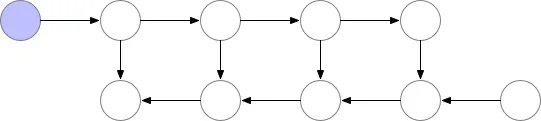
We can save a significant amount of memory by recomputing the activation values instead of storing those for large networks. The animation below shows how activation values that are stored during forward prop are consumed during backpropagation

The memory requirement scales linearly if we increase the number of nodes. During backpropagation, the activation at the $n-th$ node is consumed first (so it is independent of values in previous nodes). So we can drop storing the activation values for the previous nodes to compute the gradients for $n-th$ node. What about the gradients for $n-1$ the node? Well, we need to recompute it! That’s the trade-off we make

It is beautifully illustrated in the animation below.

In total, for every batch of samples, this approach requires $O(n^2)$ computation and $O(1)$ memory. To reduce the quadratic computational complexity, instead of dropping activation values of all previous nodes, we checkpoint some of them as shown below to bring down $O(n^2)$

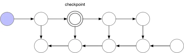
In this case, we have chosen the second node for checkpointing. Therefore, activation values for 3rd node is obtained by forward passing the values from the second node (no need to do a full forward pass from the inputs). This is illustrated in the animation below

We can combine Gradient Accumulation and Activation Check-pointing to reduce memory requirements significantly. What is the interval of dropping nodes? Well, it is recommended to drop $\sqrt{n}$ nodes if we have $n$ nodes in the network. To see the relation between node, memory and computation time, see the original article (all images were taken from there). Do remember that if we combine these approaches, it will take still more time for training than training with gradient accumulation alone.

In HF, we can simply turn it on by setting gradient_checkpointing=True while instantiating TrainingArguments.

Mixed-Precision Training

• Not all variables require FP32
• Store activation FP16 and gradient in FP32
• However, for training, load gradients in FP16.
• Modern GPUs support BF16

Once again, in HF, we can simply turn it on by setting fp16=True while instantiating TrainingArguments. Moreover, we can combine this with the above techniques!

Memory Efficient Optimizers

• Use memory-efficient optimizers such as AdaFactor, LION, 8-bit Adam, GaLore
• However, if our model gets big, we need to use distributed training using multiple GPUs!

Ref: (lengthy but well-written article from HF). I just added a running example.