Motivation
Are you wondering about the peculiar use of a sinusoidal function to encode the positional information in Transformer architecture? Are you asking why not just use simple one-hot encoding or something similar to encode positions?. Welcome, this article is for you.
Perhaps you are here after reading a few articles explaining the positional encoding function used in the Transformer architecture (proposed in the “Attention is all you need” paper) and you might be looking for some additional insights. Maybe you are redirected here after searching for an explanation about the positional encoding method in a search engine. So I am assuming that you know the working principle of various components in the transformer architecture. Even if you are currently in the learning phase, I hope you know, at the least, how the self-attention sub-layer works.
We know that adding positional information of words to the input embedding is extremely important to transformer architectures as the self-attention layer is permutation invariant (that is, the output values do not change if you change the order (position) of words in a sentence). So the fundamental question is, How to encode the positional information?. One possibility is to let the architecture learn the positional information along with the input embedding. The other method is to use fixed functions. In this article, we are going to decode and get deeper insights into the latter method.
Going by Intuition
Let us start with an example sentence: “I enjoyed the film transformers”. We generally talk about (encode) the position of the words in two ways. One is to use absolute positions as shown below. This is termed as an absolute position for the position of the words is measured with respect to a fixed position (usually the starting position) as shown in the figure below, Fig.1

Fig.1: The absolute position of words with respect to the starting word in the sequence
What we have now is the positional information represented by scalars (i.e., a single number or an index). However, recall that each word in a sentence is represented as a vector (called word embedding or input embedding) of size, 512. Therefore, in order to add these absolute positions, which are scalars, we need to convert them to a vector of the same size, 512. How do we do that? We need a mapping that takes in a scalar as input and outputs a vector of size 512. The images below show two such mappings (we restrict the dimension to 5 instead of 512 for a better explanation)

Fig.2A, Method-1: Mapping a scalar to a vector using the one-hot encoding

Fig.2B, Method-1: Mapping a scalar to a vector using the one-hot encoding
Now we have two simple and straightforward methods to encode the positional information. The first method uses one-hot encoding and the second uses broadcasting. Well, which method to use? What are the criteria to choose ?. To answer this, we need to answer two more important questions.
Question-1: Does the positional encoding method preserve the notion of distance?
Naturally, there is a notion of distance associated with the positions in a sequence. Now let us take a closer look at the distance between words in the sentence. We first use scalar representation for position to measure the distance and extend the same for vector representation. The table below shows the distance between a given word and all words in the sentence.
For example, the distance between the word the and the word I is 2 (abs(2–0))positions. Similarly, the distance between the word transformer and the word I is 4 (abs(4–0)).

Fig-3, Distance between two words in the sentence
Here is an interesting observation. Take any row, the values on the left of 0 or on the right of 0 keep always increasing (too obvious to say?). So we can say that 0 is the pivot element in any row. Let’s consider the 2nd-row corresponding to the word *the* and plot all the elements in the row. There is a perfect even symmetry at the center position ( the, in this case) as shown in the fig-4.

Fig-4, Position vs distance plot. Plotting elements in the 2nd row of fig-3. Observe the symmetry
Keep these in mind. Now, we are ready to extend the same concept to the vector representation of positions. We need the formula to measure the distance between vectors. Well, let us compute the Euclidean distance between vectors in both methods.
For the first method, where one-hot encoded representation was used to encode the position, the distance between two vectors that differ in position is always a constant 1.414 (square_root(2)) as shown in the table below. The distance is 0 only if the two vectors are the same (that’s why all elements along the main diagonal of the table are zero)!.

Fig-5, Euclidean distance between one-hot encoded position vectors
So the distance between the words I and Enjoyed is the same as the distance between I and the transformer. If you imagine plotting each row (j) one after the other, you must see a zero at the jth position and a constant everywhere else. If you find it hard to imagine, here is a plot for you (note: in this plot, the number of rows is 100, that is, we assume the max_length of a sentence is 100)
Video-1: Distance between vectors when one-hot encoding is used to represent the position of words in a sentence
However, the second method (broadcasting ) has the notion of distance. If you create a table as shown in fig-3 by computing the Euclidean distance between two vectors (words), you will see similar observations as in fig-3 (i.e., the distance for the jth position is 0 and it increases on both left and right of 0). If you plot the first row, it will look like a straight line with a positive slope. If you plot the last row, it will look like a straight line with a negative slope. At which row (or position) can we expect the even symmetry with respect to the pivot (0)? Let’s plot all the rows in the table one after the other (again, the number of rows is 100)
Video-2: Observe the shape at the starting position (0), in the middle position (50) and at the final position (100)
We can say that the first method doesn’t have a notion of distance as expected and the second method does have it. Therefore, the answer is NO to the first method and YES to the second method. Here comes the second question.
Question-2: Are the vectors encoded by both the methods orthogonal (or orthonormal)?
What? orthogonality? Why do we need to check for orthogonality? Well, before answering this question, let us step back and take a look at the vector representation of words (called word embeddings) in the embedding space. For example, consider the representation of two words ( sea, lake) in (R²) word-embedding space, as shown in leftmost figure (a) of Fig-6. Computing the dot product between these two vectors gives a value close to 1 as they are semantically closer.
Fig-6, (a:) vector representation of words in the embedding space, (b:) Direction of position vectors when using one-hot encoding, (c:)Direction of Position vectors when using broadcasting.
It is time to ask an interesting question: what happens to the result of the dot product between the two word-vectors after adding positional vectors (p0,p1)to them (assuming that sea is the first word and lake is the second word)? Look at the expressions in figure-7 below.
Fig-7,(a) dot product between word-embeddings without adding any positional information, (b)Dot product after adding positional vectors (p0,p1)to the word-embedding
We ideally want the dot product of position vectors (p0 and p1) to be zero (in other words, we do not want to change the original score between the two vectors w_0 and w_1). This is possible if and only if all the position vectors are orthogonal to each other. Therefore, as you can see from figures (b) and (c:)of Fig-6, the dot product between any two position vectors represented using a one-hot encoding scheme is zero, whereas the dot product between any two vectors represented using a broadcasting scheme is zero if and only if one of the vectors, say p_0, is a zero vector. Moreover, all the position vectors represented by the broadcasting scheme align in the same direction (i.e., they are a subspace spanning a line in n-dimensional vector space, just a boasting :-)
Therefore, the answer is YES to the first method and NO to the second method.
Problem: So we got into trouble. We need to choose either the first method if orthogonality is required or choose the second method if the notion of distance is required. However, we need a method that has both these properties. Does it exist?
Orthogonal functions
Well, I am gonna stretch the length of this article a bit to explain the characteristics of sinusoids. Sinusoids are characterized by two parameters, amplitude and wavelength(frequency).

The amplitude of the sine wave varies between +1 to -1. The frequency (number of cycles in a fixed interval) varies from zero to infinity. The wavelength is inversely proportional to frequency (that is, increasing wavelength means decreasing frequency). The figure below, Fig-9, shows two sinewaves of two different wavelengths. Notice that as the wavelength increase from pi to 2*pi, the frequency decreases.

Fig-9, sinewaves with two different (wavelength) frequencies
The equation for the red wave is sin(1x) and for the blue wave is sin(2x). Here comes the interesting fact. Now we have a distance associated with the wavelengths! The wavelength can be increased progressively from 0*pi, 1*pi, 2*pi, 3*pi, … ,20000*pi. The wave of 3pi wavelength is close to 4pi than to 5pi (in the infinite-dimensional real vector space). So our first requirement, the distance should increase proportionally if an *ith position moves further from a fixed *jth* position, is satisfied (to some extent).

Fig-10, sinewaves of Increasing wavelengths
The next important requirement is orthogonality. We know sine and cosine are orthogonal as they differ by 90⁰ angle (that’s just a visual proof). However, what about the orthogonality for two sine waves of different frequencies (or wavelengths)?. They are orthogonal (in the infinite-dimensional real vector space)!. Wow, we found a function that satisfies both the requirements and is also extendable to a sequence of any length. This is really amazing!. Whatever that we learned for sine waves is equally applicable for cosine waves. Here is the formula that makes use of the sinusoidal functions as shown below,

Fig-10. the positional encoding function for the jth position ( row in the table) and ith dimension (column in the table)from the paper
Well, what is the significance of the cosine part?. To answer this question, we need to think a little about the caveats of using sine waves alone. In the previous toy example, we just learnt that for the position j=0 (a row in the table), we don’t want the row full of zeros. Given that we are using sine waves that have many zero crossings, we might end up with rows full of zeros. To avoid this, we need to interleave (or concatenate) the cosine waves. Therefore the amplitude cosine becomes +1 or -1 whenever the amplitude of sine becomes zero.
One more fact is that the sine waves need not necessarily start from 0 (as in the case of absolute position encoding), it can be offset by k units as shown in figure 11. The offset is represented as a linear function ( x+4, in this specific example) of sine. Therefore, the same method can also be used for relative positional encoding
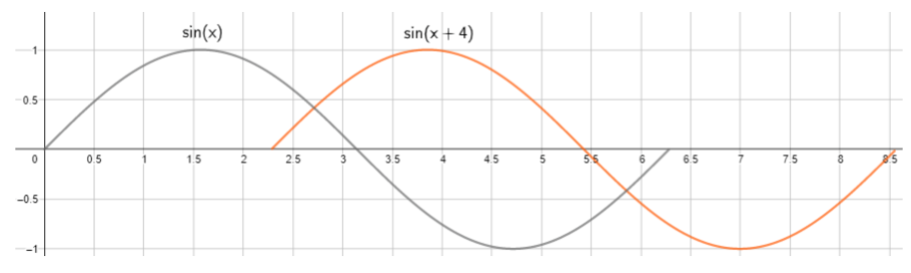
Fig-11, Functions of same wavelength offset (delayed) by k=4 units
Let’s do a quick sanity check by plotting the position vs distance curve and position vs dot product curve for the sinusoidal scheme. To compute the dot product or distance, we need two vectors. We start with the 0th (jth position in general) position vector and compute the distance and inner product with itself and the rest of the position vectors. This generates a graph. Repeat this for the rest of the positions. Capture all these plots as frames and compile them to create animations as shown below.
Animation of Position vs distance curve
Animation for Position vs inner product curve
Well, that’s all I have to share with you. I hope this article has shed some light on the positional encoding method used in the transformer architectures. Happy learning!.